FRS

Filtered Rayleigh Scattering (FRS)
The non-intrusive Filtered Rayleigh Scattering (FRS) method is well suited to measure the temperature, velocity, density and pressure in unseeded gas flows. It was developed and proved by DLR. The light source is a high power cw-Laser with a precisely adjustable wavelength. The Laser is used to create a light sheet with a homogenous intensity distribution over the entire cross-section. The FRS method is based on the acquisiton of the intensity of the Rayleigh scattered light from gas molecules in a laser light sheet spectrally filtered by a molecular filter, a iodine cell. The absorption spectrum of iodine is used to eliminate the scattered light of walls and Mie scattered light. The intensity signal in the light sheet is then focused on a sCMOS chip behind the iodine cell.
The shape of the frequency spectrum is influenced by flow field parameters temperature, pressure, Doppler shift and the composition of the gas. Knowing the composition of the gas and the exact shape of the iodine absorption spectrum therefore enables determining the parameters temperature, pressure, velocity and density by using the Tenti model. To gain the information needed for the model to reconstruct the flow parameters the laser frequency is varied systematically in equidistant steps (Fig.3), which is called Frequency Scanning-FRS (FSM-FRS).
Figure 1 shows the FRS measurement setup of a heated free jet. Main objective of the measurement was to determine the temperature distribution in the stream and to compare the FRS measured temperature with that of a calibrated PT100 temperature probe. The results are shown in Figure 2. The temperature distribution in the FRS graph on the left is spatially highly resolved whereas the PT100 graph shows an averaged temperature distribution due to the interpolation of 147 individual measuring points distributed over the entire measurement range. The temperature averaged over 10 pixels in the core stream and in the surrounding area show very similar results in both measurements with less then 0,4% deviation.
The FRS method uses the elastic light scattered from molecules and does not need additional particles in its setup. This fact makes it interesting for environments where seeding particles cannot be added easily or where there are few particles in principle (e.g. cryogenic wind tunnels). Other applications are small regions of interest where a measuring probe would negatively interfere with the gas flow, turbulent and high temperature flows (100-2000K) and of course measurements where the various flow quantities should be acquired with only one simple setup. Furthermore the proportional dependence of the intensity in the Tenti model on pressure makes FRS especially suited for high pressure environments (e.g. combustion chambers, turbomachinery).
The ILA R&D FRS system consists of the high power laser source, a wavemeter, lightsheet optics, the FRS camera module with the iodine filter (Fig. 4), the INDIO Controller and an FRS PC. All hardware signals come together in the INDIO Controller, which controls i.a. the wavelength, light sheet, laser power and iodine cell temperature. All of this is incorporated in the ARES-Software, which offers a comprehensible design, full control of all settings and easy-to-follow steps that are necessary for performing measurements.
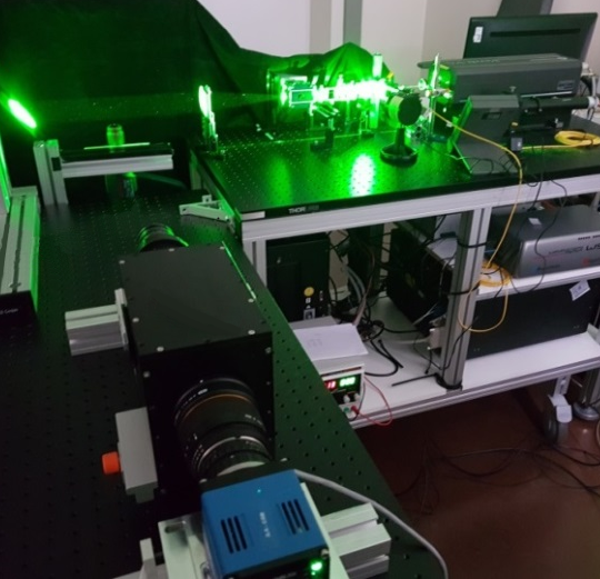
Fig. 1: FRS mesurement setup with Laser and Camera Module.
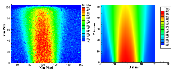
Fig. 2: Comparison of the FRS temperature measurement (high spatial resolution) with a averaged PT100 measurement in a free jet.
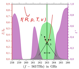
Fig. 3: Convolution of the intensity of the rayleigh scattered light with the filter curve of the iodine cell.
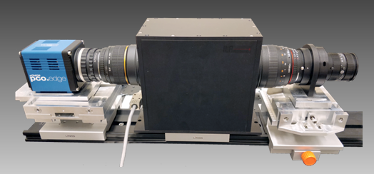
Fig. 4: Camera modul with iodine cell.
FRS for the investigation of intake flows in aircraft turbines
In the development of novel aircraft concepts, the reduction of fuel consumption and emissions is an important aspect. In this context, new concepts are being developed that integrate the engines into the aircraft body. This causes, e.g. due to boundary layer flows, disturbed steady-state and transient inflows to the engines, which significantly affect their aerodynamic load and operational behavior.
In the EU research project SINATRA “Seeding free non intrusive aero engine distortion measurements”, the possibility of using the Filtered Rayleigh Scattering technique (FRS) for seeding-free investigation of inlet flows in engines on the test bench and potentially in flight tests is therefore being investigated. To this end, FRS measurements are first performed on a simplified flow experiment in order to optimize the experimental setup, characterize the measurement system and determine the measurement uncertainty. In a second step, FRS measurements of the pressure and velocity field are performed on a test rig designed for the investigation of engine intakes at Cranfield University.
The simplified experimental setup (Figure 5) consists of a conditioned pipe flow with an inner Diameter di= 80mm. In this measuring cross-section flow velocities of approx. 30 to 100 m/s can be generated. Optical access is provided by an anti-reflective-coated glass tube. The laser light sheet is coupled in via a slit in the glass tube.
Figure 7 displays the unifying image fiber bundle used to observe the flow from six perspectives. The active area on the inlet of each of the six fiber arm is 4x4mm with about 50000 individual fibers. The inlet of each 3m fiber arm is equipped with an adjustable fiber objective. The outlet of the fiber bundle has an active area of 12×8 mm, thus allowing to capture 6 perspectives with only one camera module. This setup allows for measurements in environmental challenging environments: the delicate camera module can be placed in a protected location up to 3m away from the object.
The fiber heads are mounted on adjustable magnetic lab stands, allowing for fast alignment and adaption of perspectives according to the experimental requirements. The optical setup results in an optical resolution of about 1mm in the ROI for the depicted setup.
The outlet of the fiber bundle is attached to a bespoke camera module consisting of a temperature stabilized molecular filter (iodine cell) and an pco.edge 4.2 sCMOS camera with a resolution of 2048×2048 pixel for aquiring the image data.
The observation perspectives for the experiments have been selected according to the optimization frame work developed byDoll, Röhle, & Dues (2022) and Doll, Röhle, Dues, & Kapulla (2022).
Due to the inlet configuration consisting of flow straightener, a contraction and a relatively short distance to the measuring cross-section, a fully developed pipe flow profile is not available at the region of interest (ROI). Instead a ’flat-top’ profile is expected.
To validate the FRS measurements, the velocity field in the pipe is recorded on a dense grid for three operating points using a calibrated Laser Doppler Velocimetry (LDV).
Figure 8 shows the velocity profile measured with FRS for three operating points in comparison to the velocity profiles measured with LDV (Doll et al. (2023)). In the center region of the flow, the flow profile is strongly flattened in both the LDV and FRS measurements, while a flowgradient occurs in the edge region due to the boundary layers that build up. In the center area, the difference between the FRS and LDV measurements is less than 1more sharply, but this can be explained by the measurement position of the LDV measurement further downstream.
To allow the simultaneous determination of three velocity components, the pressure and the static temperature, the measurement cross-section is viewed from six perspectives through a 6-arm image fibre bundle with about 50000 fibres per arm and imaged onto the sensor of the camera.
For the undisturbed flow case the comparison of the FRS velocity results with LDA measurements shows a very good agreement with deviations less than 1%.
In the next step, measurements were made behind a swirl generator (Figure 10), which was first installed 0.25 D and then approx. 7 D upstream of the measurement cross section.
Figure 11 shows the measured 3C velocity distribution approximately 20 mm behind the swirl generator for the operating point of 30m/s 100m/s (10V). For this operating points, the circumferential components of the velocity in the secondary flow are clearly visible. Even the wake dents of the four swirl vanes are well identified, especially in the distribution of the axial component w. In the centre of the flow field, a backflow region is evident.
To test the FRS temperature measurement, hot air with comparatively low velocity was fed through a glass tube into one of the swirler’s passages. Compared to the corresponding results in Figure 11, a lower velocity region is clearly visible in the axial velocity component w in a partial segment behind the swirl generator (Figure 10). The contour drawn corresponds to the zone of increased temperature due to the hot gas injection. The contour drawn corresponds to the zone of increased temperature (Figure 12) due to the hot gas injection.
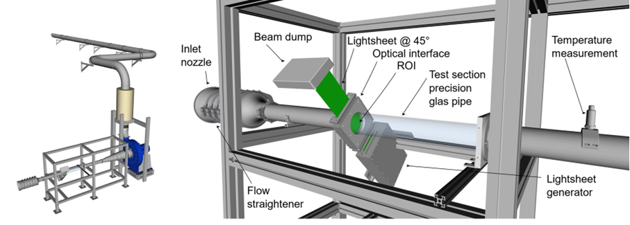
Fig. 5: Test rig for the investigation of pipe flows
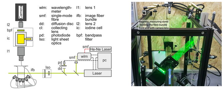
Fig. 6: Components of the FRS measurement system with image fibre and installation at the test rig
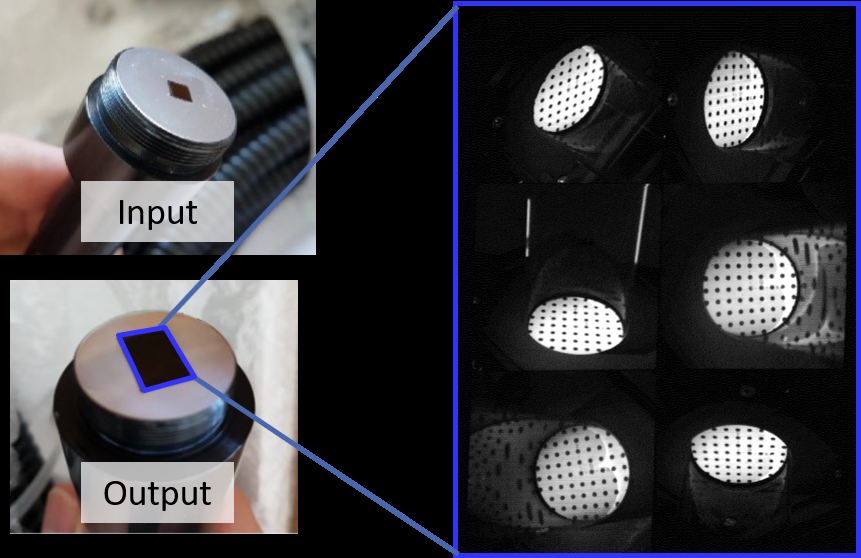
Fig. 7: Input and output view of the six to one imagefiber bundle used to oberserve the scene simultaneously from different perspectives (left). Resulting image for observation of a calibration target (right).
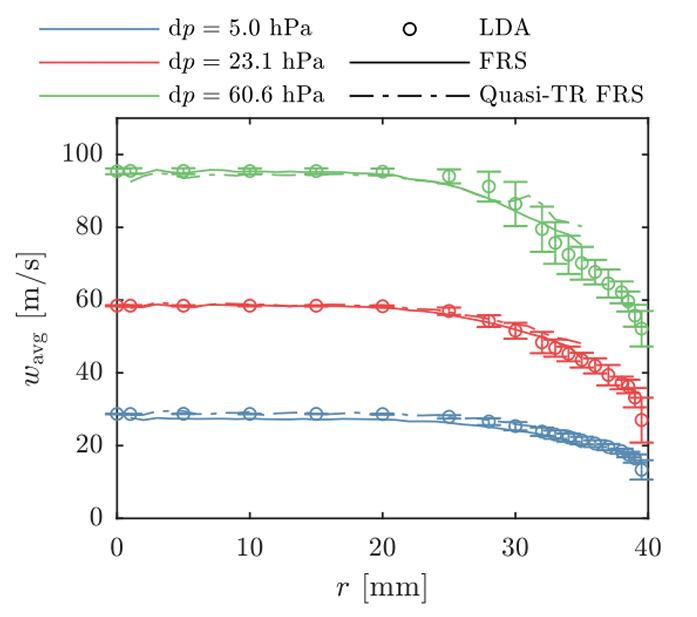
Fig. 8: Comparision of the FRS-derived values for axial velocity with the reference values provided by the test rig, resp. LDA measurements.
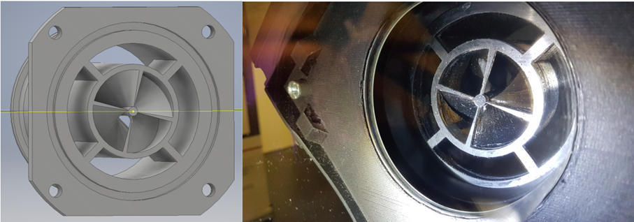
Fig. 9: Swirl generator with four channels for installation in the test bench
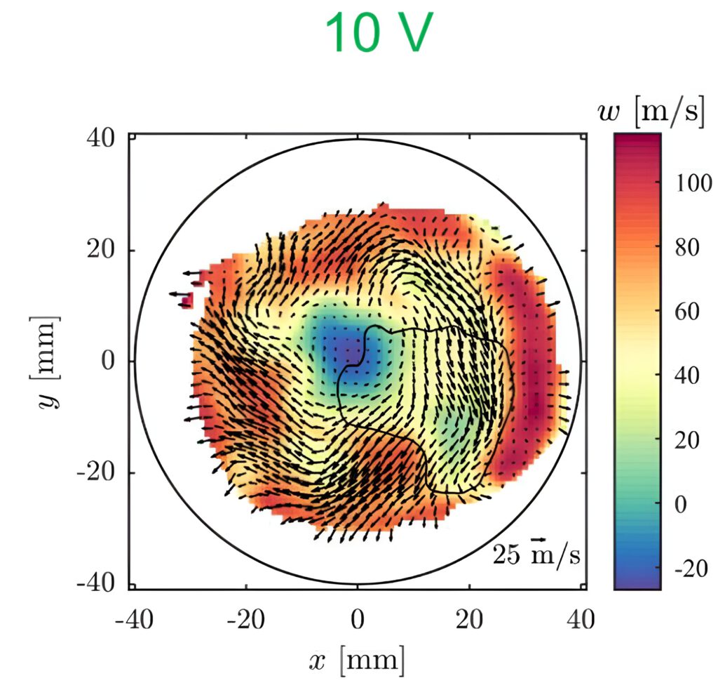
Fig. 10: Velocity distribution 20 mm downstream of the swirl generator with warm air blown in one channel
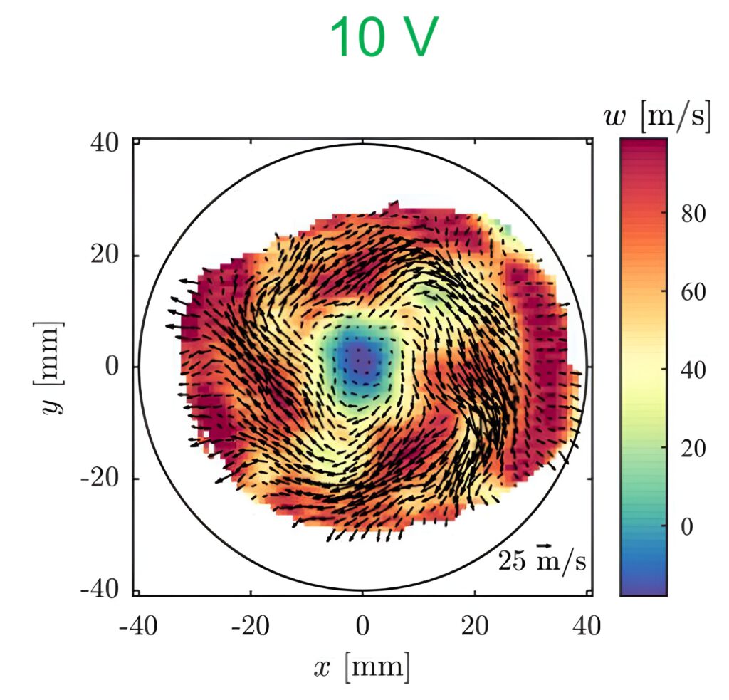
Fig. 11: Velocity distribution 20mm behind the swirl generator
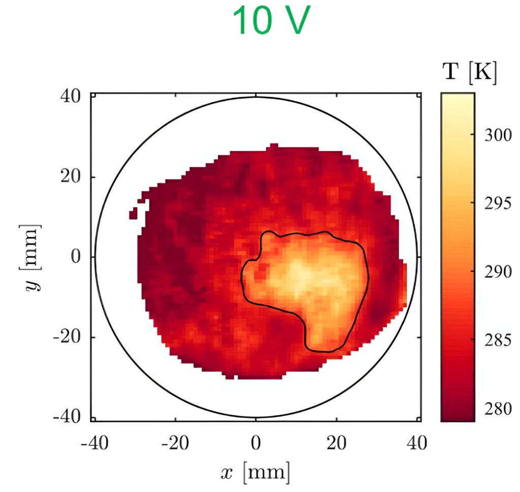
Fig. 12: Temperature distribution 20 mm downstream of the swirl generator with hot air blown in one channel
Complex Intake flow setup
The Cranfied Complex Intake Test Facility (CCITF) provides a experimental platform for the analysis of engine intakes. It is capable of producing internal flows up to a Mach number of 0.6. In frame of the SINATRA project a „high-offset“ S-Duct diffuser configuration was choosen as reference experiment. More Information on the CCITF can be found in Migliorini et al. (2024). A overview about the geometric setup is given in Figure 13.
The internal diameter of the optical test section is 160 mm. The measurement plane was placed close to the outlet of the S-Duct. A bespoke light sheet interface enabled the illumination of the ROI with the laser. The available light sheet could illuminate approximately half of the cross section, therefore each experiment was conducted once with the lightsheet traversed to the respective upper and once traversed to the lower part of the ROI. The FRS measurements where then evaluated for each part, the resulting fields were stitched together via software.
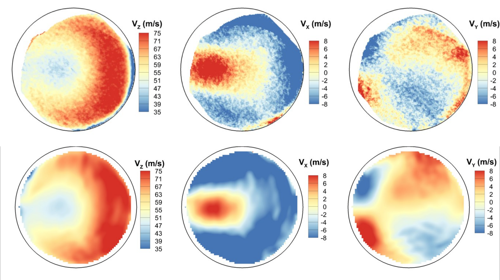
During the FRS measurement campaign the following flow conditions where examined: 0.18, 0.27 and 0.4 Mach at the ROI. The resulting velocity fields are depicted in Figure 14. The axial velocity profile is skewed with higher velocities on the right side of the ROI due the s-duct inlet. The formation of the secondary flow (dean vortices) is clearly observable. About 80independently from 6 perspectives. Due to the multi image-fiber approach it is possible to observe almost the entire crossection with multiple perspectives, thus allowing for robust measurements even though some regions are inherently blocked or shaded due to experimental constraints on individual fiber heads.
A measurement campaign with time-averaged Stereo Particle Image Velocimetry (S-PIV) was conducted by Cranfield University to generate benchmark data for the FRS velocity measurements. The S-PIV system used two SCMOS cameras with a resolution of 1280 by 800 pixel at 8 kHz. The resulting spatial resolution in the ROI is in the order of 2.3 mm. DEHS seeding with an nominal diameter of 1 μm was illuminated by an pulsed ND:YAG laser. 20000 flow-fields were captured and averaged to create the reference data set (Figure 15).
Our latest research on Filtered Rayleigh Scattering (FRS) has recently been published on our website and can be viewed here: ila-rnd.com/frs-dgv
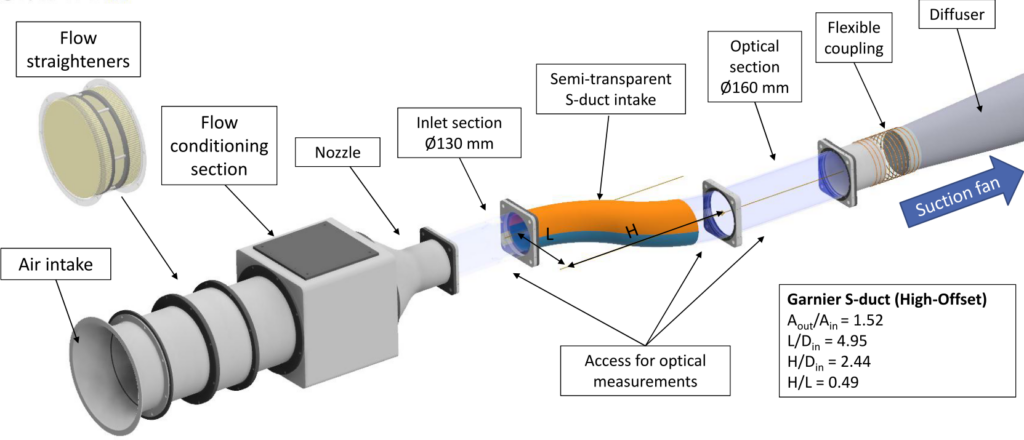
Fig. 13: Rendering of the Cranfield Complex Intake Test facility (CCITF).
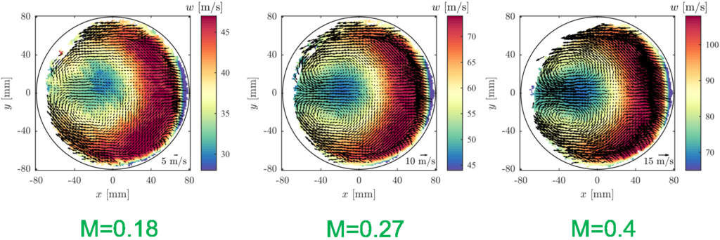
Fig. 14: Axial velocity field obtained with FRS at the CCITF at 0.18 Mach (left), 0.27 Mach (center left) and 0.4 Mach (center right). The in-plane components are denoted with black arrows. The number of valid perspectives is drawn as insert (right).